04 State Estimation & Filters · #21 of 46

Kalman Filter

The math that flew Apollo to the Moon

You have two clocks. One runs fast, one runs slow, and neither is right. What time is it?

The wrong answer is "pick the better clock." The Kalman filter's answer, provably the best answer in the universe, is a single number that splits the difference, weighted by exactly how much each clock lies.

A robot is always holding two clocks: what it predicts from its own motion, and what it measures from a noisy sensor. The filter below fuses them in one dimension. The muted line is the truth the robot can't see; the yellow dots are noisy GPS fixes; the accent line is the filter's belief, wrapped in a shaded band of doubt.

● PREDICT — coasting K=0.00 err=0.00m σ=0.00

GPS interval 0.5 s meas σ² (R) 0.30 proc σ² (Q) 0.04 speed 1.0×

Drag on the canvas to inject a manual GPS fix. K→1 trusts GPS, K→0 trusts odometry.

Try this:

Watch the band breathe. It swells between GPS fixes (every blind step adds doubt) and snaps tight the instant a yellow dot arrives. That pulse is the whole algorithm.
GPS blackout. Push the GPS interval to 5 s. Watch the estimate drift and the band balloon. This is what a tunnel does to your phone.
Garbage GPS. Crank the measurement σ² up. The filter shrugs, trusts its own motion, and barely flinches at each dot.
Perfect GPS. Drop the measurement σ² near zero. Now the filter snaps onto every dot like a magnet. Same equations, opposite personality.

The dial you're turning, implicitly, is trust. The filter computes it for you, every single tick, optimally.

The one number that runs everything

Last phase we faked sensor fusion by guessing a blend factor: alpha = 0.98, trust the gyro a lot, the accelerometer a little. It worked, but why 0.98? What happens when the floor turns to ice and the gyro starts lying?

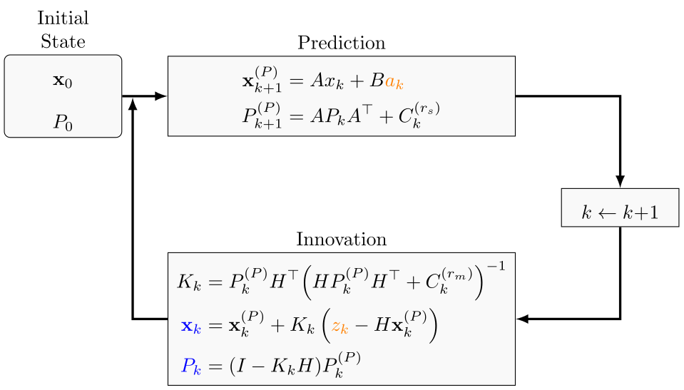
The Kalman filter refuses to guess. At every instant it asks one question, who do I trust more right now?, and answers with a number called the Kalman gain, $K$ . When your sensor is garbage, $K \to 0$ and the filter leans on its own prediction. When your prediction is garbage, $K \to 1$ and the filter snaps to the sensor. It recomputes this a hundred times a second, and the value it lands on isn't a heuristic. For a linear system with Gaussian noise it is optimal: the single best estimate the laws of probability permit. No filter can ever beat it.

The Kalman filter loop: a predict step projects the state and grows uncertainty, then an update step folds in a measurement and shrinks uncertainty, feeding back into the next predict. — The eternal two-step. Predict pushes the estimate forward and inflates the doubt; update folds in a measurement and deflates it. The arrow loops back forever. · MartinThoma, CC BY-SA 4.0

Driving through a tunnel

Picture yourself in a tunnel with the radio on.

Predict (the speedometer). It reads 60 mph, so you reason: one more minute, one more mile. Smooth, instant, always available, and quietly wrong, because tires slip and the road curves. Your uncertainty bubble inflates. 🎈

Update (the GPS). You burst out of the tunnel and the GPS barks "Exit 4." It's noisy, but it's an anchor to the real world. Your bubble deflates. 🤏

The Kalman gain is the referee between them. Trust nobody completely; trust everybody exactly as much as they've earned. That's the entire trick, and it's why your phone can hold a believable blue dot through a tunnel where it can't see a single satellite.

Portrait of Rudolf E. Kálmán, inventor of the Kalman filter. — Rudolf E. Kálmán · 1930–2016 His 1960 filter turns noisy measurements into *provably optimal* estimates, and flew Apollo to the Moon. read more →

A two-hundred-year-old idea

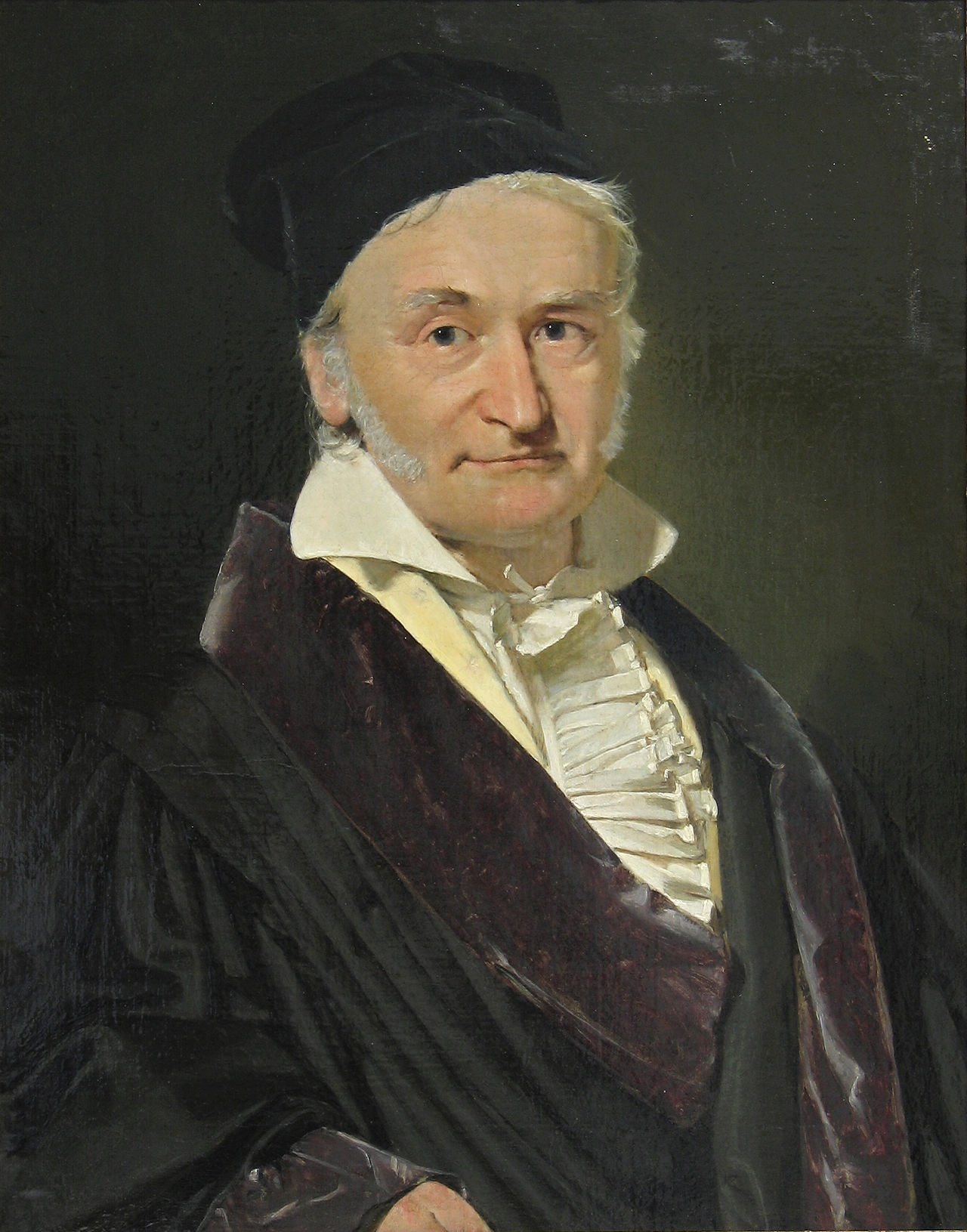
The filter feels modern, but its heart is older than the lightbulb. In 1801 the astronomer Piazzi spotted a new object, the asteroid Ceres, then lost it behind the Sun's glare. A few scattered, error-riddled observations were all anyone had. A 24-year-old named Carl Friedrich Gauss invented the method of least squares to wring the most probable orbit out of that noisy scatter, predicted exactly where Ceres would reappear, and astronomers found it. The Kalman filter is least-squares made recursive: Gauss's idea, run forward in time, one measurement at a time.

Portrait of Carl Friedrich Gauss, who invented the method of least squares. — Carl Friedrich Gauss · 1777–1855 Invented least-squares at 24 to recover the lost asteroid Ceres, the Kalman filter's direct ancestor. read more →

The two laws

Strip away the matrices and only two laws remain, and you've already watched both in the demo:

Predict always grows uncertainty. Moving blind can only ever make you less sure.
Update always shrinks it. A measurement, however noisy, can only ever make you more sure.

Predict, update, predict, update: the same heartbeat as every estimator in this course, now with the trust factor computed optimally instead of guessed.

The five equations, and where the gain comes from

The filter tracks a state estimate $\hat{x}_k$ and its covariance $P_k$ , the size of the uncertainty bubble. Each tick runs two stages.

Predict: project the state forward through the motion model $F$ , with control $u_k$ , and inflate the covariance by the process noise $Q$ :

\hat{x}_k^- = F \hat{x}_{k-1} + B u_k

P_k^- = F P_{k-1} F^{\mathsf{T}} + Q

Update: compute the gain, correct the estimate by the measurement residual, and deflate the covariance:

K_k = P_k^- H^{\mathsf{T}} \left( H P_k^- H^{\mathsf{T}} + R \right)^{-1}

\hat{x}_k = \hat{x}_k^- + K_k \left( z_k - H \hat{x}_k^- \right)

P_k = \left( I - K_k H \right) P_k^-

Read the gain $K_k$ as a ratio of doubts: my prediction's uncertainty over prediction plus measurement uncertainty. When the sensor is noisy ( $R$ large), $K_k \to 0$ and the correction term vanishes, so trust the prediction. When the prediction is shaky ( $P_k^-$ large), $K_k \to 1$ and the estimate jumps to the measurement. The symbols:

$\hat{x}_k$ : state estimate (e.g. position, velocity)
$P_k$ : covariance (the uncertainty bubble)
$K_k$ : Kalman gain (the trust factor, computed, never guessed)
$Q$ : process noise (doubt added by motion)
$R$ : measurement noise (how much the sensor lies)
$F$ : state transition (the motion model)
$H$ : measurement matrix (how the sensor sees the state)

In the demo, the reported error is $|\,x_{\text{true}} - \hat{x}\,|$ and the band's half-width is $\sqrt{\lambda_{\max}(P)}$ , the largest eigenvalue of the covariance, the longest axis of the doubt ellipse.

Build the 1D filter from scratch

In one dimension the matrices collapse to scalars and the whole filter fits in a struct:

struct KalmanFilter1D {
    x: f32, // state estimate
    p: f32, // variance (uncertainty)
    q: f32, // process noise
    r: f32, // measurement noise
}

impl KalmanFilter1D {
    fn predict(&mut self, u: f32) {
        self.x += u;      // motion model
        self.p += self.q; // uncertainty grows
    }

    fn update(&mut self, z: f32) {
        let k = self.p / (self.p + self.r); // Kalman gain
        self.x += k * (z - self.x);         // correct toward measurement
        self.p *= 1.0 - k;                  // uncertainty shrinks
    }
}

That let k = self.p / (self.p + self.r) is the entire idea: the same ratio of doubts as the matrix version, with the transpose and inverse stripped away.

To take it to a real rover, hand an LLM this brief: implement a 2D Kalman filter in Rust fusing GPS (x, y) at 1 Hz with R = [[10,0],[0,10]] and IMU velocity (vx, vy) at 100 Hz with Q = [[0.1,0],[0,0.1]], state vector [x, y, vx, vy], targeting a Raspberry Pi via the rppal crate. For the sensor side, a u-blox NEO-M9N gives roughly 1.5 m accuracy over UART, while a \$40 Adafruit Ultimate GPS is fine for learning. Parse its $GPGGA NMEA sentences for lat/lon, fix quality, and HDOP, then project to local XY with UTM.

Run the filter yourself

The entire filter is the eight lines below, and it is editable. Change q (process noise) and r (measurement noise), then run it again: push r up and the gain stays small so the filter leans on its own prediction; drop r and the estimate snaps onto every measurement.

1D Kalman filter editable · Python

x, p = 0.0, 1.0
q, r = 0.01, 0.25
measurements = [0.39, 0.50, 0.48, 0.29, 0.25, 0.32, -0.66, 0.20, 0.31, 0.49]
for k, z in enumerate(measurements):
  p = p + q
  K = p / (p + r)
  x = x + K * (z - x)
  p = (1 - K) * p
  print(f"{k}: z={z:+.2f} est={x:+.3f} K={K:.2f}")
print()
print(f"final estimate {x:.3f} (truth is about 0.0)")

ready

Two clocks, neither right. A 24-year-old chasing a lost asteroid with a pencil. A rejected paper that ended up steering a spacecraft to the Moon. They are all the same idea, seen from different centuries: when you cannot know the truth, weigh your guesses by exactly how much each one lies, and the math will hand you the best answer there is.

Your phone is doing it right now, holding your blue dot steady through the tunnel.