04 State Estimation & Filters · #20 of 46

Complementary Filter

Two sensors that lie in opposite directions, and the one line of code that makes them tell the truth

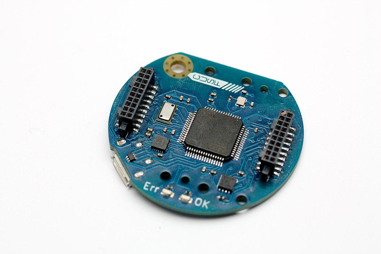
A drone avionics / flight-controller board. — A drone flight controller fuses a noisy accelerometer and a drifting gyroscope on one board: the complementary filter, in hardware. · Adam Greig, CC BY-SA 2.0

A gyroscope is the eyewitness who remembers every second perfectly but can't tell you what happened an hour ago. An accelerometer is the drunk who shouts the right answer (and three wrong ones) every second.

Neither can be trusted alone. So we make them police each other.

This is your first taste of sensor fusion: taking two flawed sensors and blending them into one estimate that is better than either. Below is the whole drama on one canvas. The faint line is the truth your robot is trying to track. Red is the accelerometer: roughly right, violently jittery. Blue is the gyro: silky smooth, slowly peeling away from reality. The accent line is the fused estimate, and it's the only one you'd ever trust.

α (blend) 0.96 σ (accel noise) 0.18 drift (gyro drift) 0.00

Raise σ to make the accel trace jitter, raise drift to make the gyro trace wander off. Watch the fused estimate stay near truth.

Try this:

Trust the gyro completely. Set α = 0.99 and wait 30 seconds. The fused line glides beautifully, straight off the truth. That's drift, integrated.
Trust the accelerometer completely. Set α = 0.50. Rock-stable on average, but it shivers like the red line. That's noise, unfiltered.
Find the sweet spot. Try α = 0.96. Smooth and anchored. You just did sensor fusion.
Shake it. During fast tilts, notice the fused line tracks the smooth gyro; when things settle, it quietly slides back toward gravity. The handoff is the whole trick.

Why each sensor lies

The gyro and the accelerometer fail in opposite frequency bands, and that is the entire reason this works.

A gyroscope measures angular velocity, how fast you're turning right now. To get an angle, you integrate it over time. Integration is unforgiving: a microscopic, constant bias of a fraction of a degree per second gets summed up forever, and within a minute your "angle" has wandered off into fiction. Precise over a second, hopeless over a minute.

Orientation is three turns: yaw, pitch, and roll, one per ring. The bright triad at the core is the body's own axes; watch them rock back and forth. The dashed arrow is gravity, pinned pointing down: however the body tilts, an accelerometer always recovers that direction, while a gyro only feels how fast each ring is turning right now. Fuse the steady down-vector with the fast turn-rates and you know exactly how the body is tilted.

An accelerometer measures acceleration, and the biggest, most reliable acceleration around is gravity: a steady 1 g pointing straight down. So an accelerometer always knows which way is down, which means it always knows your true tilt on average. The catch: it can't tell gravity apart from the robot's own motion. Every bump, vibration, and quick jerk shows up as a spike. Never drifts, always noisy.

The one line that fuses them

The trick is to high-pass the gyro (keep its fast, trustworthy changes; throw away its slow drift) and low-pass the accelerometer (keep its steady down-vector; throw away its jitter), then add the two. Remarkably, that entire idea collapses into a single update:

\theta_{n} = \alpha \,\bigl(\theta_{n-1} + \omega\,\Delta t\bigr) + (1 - \alpha)\,\theta_{\text{accel}}

Read it left to right. The term $\theta_{n-1} + \omega\,\Delta t$ is the gyro's prediction: take last frame's angle and add this frame's rotation. The term $\theta_{\text{accel}}$ is the accelerometer's raw tilt, $\arctan2(a_y, a_z)$ . The knob $\alpha$ (typically 0.96 to 0.99) decides how much you lean on the smooth-but-drifting prediction versus the noisy-but-honest correction. High $\alpha$ trusts the gyro for the short term; the small $(1-\alpha)$ slice of accelerometer is just enough to nudge the drift back to ground truth, forever.

Where it runs

This exact filter is on the flight controller of nearly every consumer drone (Betaflight, ArduPilot, PX4) running anywhere from 1000 to 8000 times a second to keep the horizon level while the motors scream. Variations of it stabilize the camera in your phone and the gimbal on an action cam. It is, quite possibly, the most-deployed sensor-fusion algorithm on Earth, and it is one line long.

From spacecraft to your pocket

The same gyro-plus-accelerometer pairing once filled a box the size of a basketball. The Apollo guidance system carried an inertial measurement unit whose parts had names that sound like a 1960s sci-fi script: the gyros were Inertial Reference Integrating Gyros and the accelerometers were Pulse Integrating Pendulous Accelerometers. That hardware steered men to the Moon and back. The trick that shrank it into your phone was MEMS, microelectromechanical systems: tiny gyroscopes and accelerometers etched into silicon, the same way chips are made. Once an IMU cost a few dollars and a few square millimeters, it went everywhere. Almost every smartphone and tablet has one. So do fitness trackers, the Nintendo Wii Remote, and the Segway, whose entire balancing act is an IMU refusing to let you fall over. Cheap MEMS IMUs are also what made the whole consumer drone industry possible.

Why α picks a cutoff frequency, and how to choose it

The complementary filter is a first-order high-pass on the gyro path and a first-order low-pass on the accelerometer path, sharing one crossover. That crossover sits at the cutoff frequency:

f_c = \frac{\alpha}{2\pi\,\Delta t\,(1-\alpha)}

For $\alpha = 0.98$ at 100 Hz ( $\Delta t = 0.01\,\text{s}$ ):

f_c = \frac{0.98}{2\pi \times 0.01 \times 0.02} \approx 0.78\ \text{Hz}

Read it physically: anything changing faster than about 0.78 Hz (vibration, a fast tilt) is trusted to the gyro; anything slower (steady gravity, accumulated drift) is trusted to the accelerometer. Notice $\Delta t$ in the denominator: halve your loop period and $f_c$ doubles, even though α never moved. That's why α and sample rate must be tuned together.

To gauge how lost the gyro alone gets, you can track the absolute error against ground truth: $\lvert \theta_{\text{true}} - \theta_{\text{gyro}} \rvert$ climbs without bound, $\lvert \theta_{\text{true}} - \theta_{\text{accel}} \rvert$ stays bounded but ragged, and the fused error stays both bounded and smooth. The demo plots all three so you can watch the trade.

The whole loop, in real code, is barely longer than the equation:

struct ComplementaryFilter {
    angle: f32,
    alpha: f32,
}

impl ComplementaryFilter {
    fn update(&mut self, gyro: f32, accel_angle: f32, dt: f32) -> f32 {
        let gyro_prediction = self.angle + gyro * dt;
        self.angle = self.alpha * gyro_prediction + (1.0 - self.alpha) * accel_angle;
        self.angle
    }
}

where accel_angle comes from the gravity vector, accel_y.atan2((accel_x.powi(2) + accel_z.powi(2)).sqrt()). Wire it to a $2 MPU6050 over I2C, calibrate the gyro bias once at startup, and you have a self-leveling angle estimate.

Key takeaways

The gyro is precise over a second but drifts over a minute; the accelerometer is noisy but always knows which way is down. Their errors live in opposite frequency bands.
The complementary filter high-passes the gyro and low-passes the accelerometer, then adds them, often a single line of code.
α and your loop rate together set a cutoff frequency. Tune them as a pair, not in isolation.
It's the cheap cousin of the Kalman filter: no matrices, runs on an 8-bit chip, and it flew hobby quadcopters long before fancier estimators were affordable.

Two sensors, each confidently wrong in its own way. Alone, one wanders off and the other can't sit still. But press them together at the right frequency and their lies cancel: the drift gets pinned to gravity, the jitter gets smoothed by motion, and what falls out the other side is a steady, honest angle.

That is the quiet promise of sensor fusion, and it begins with one line of arithmetic: trust nobody completely, and you'll find the truth between them.