Poles & Zeros

A transfer function is a fraction of polynomials in the complex variable $s$. The roots of the denominator are the poles: the system's natural modes, the frequencies and decay rates it falls into when you stop forcing it. The roots of the numerator are the zeros, which don't create motion of their own but reshape how the poles' motion comes out. Poles are the engine; zeros are the gearbox.

Drag the poles yourself

The left pane is the complex $s$-plane. The two × marks are a conjugate pole pair, and the red shaded region on the right is the forbidden zone. The right pane is the step response, recomputed every single frame as you drag. Move the poles around and watch the system's mood change in real time.

Drag the poles

reset

status —

underdamped critical overdamped unstable

ζ (damping) —

ω_n (natural frequency) —

dominant τ —

poles —

what to try

• Drag a pole horizontally toward the imaginary axis. Watch the decay get slower and the envelope swell.
• Drag a pole across the imaginary axis (into the red zone). The trace explodes: the system is now unstable.
• Bring the two poles toward the real axis. The conjugate pair collides, and you've reached critical damping, the fastest non-oscillating response. Continue past it: two real poles, slower than critical.
• Slide a pole up the imaginary axis (purely imaginary). The response becomes a pure sinusoid: undamped natural oscillation at ω_n.

Two coordinates tell the whole story. How far left a pole sits (its negative real part) is the decay rate: far left means the system forgets a disturbance fast, hugging the imaginary axis means it lingers forever. How high a pole sits above the real axis is the ringing frequency: pull it up and the response oscillates faster on its way to the target.

Bring the conjugate pair down onto the real axis and they collide at critical damping, the fastest you can settle without a single wobble of overshoot. Push past that and you get two separate real poles, sluggish and overdamped, like a door closer that takes its sweet time.

A pole that sits close to the imaginary axis does not just ring longer. It also makes the system dangerously eager to ring at one particular frequency. Drive it with a sine wave whose frequency happens to match the pole's height, and the response swells far past the size of the push. That is resonance, and it is the same effect that lets a singer crack a wine glass or a gust of wind set a bridge swaying.

↘ Why a near-axis pole sings: the gain blows up at one frequency

Feed a system a steady sine wave at frequency $\omega_0$ and the steady-state output is just the input scaled by the gain $G$. For a single pole at $s_P = \sigma_P + j\omega_P$, that gain works out to:

$$G(\omega_0) = \frac{1}{\sqrt{\sigma_P^2 + (\omega_P - \omega_0)^2}}$$

Look at the denominator. The gain is largest when the driving frequency $\omega_0$ lands right on the pole's height $\omega_P$, because the second term vanishes and you are left dividing by $\sigma_P$ alone. So the peak response happens at the ringing frequency, exactly where you would guess from the demo.

Now slide the pole toward the imaginary axis, shrinking $\sigma_P$. The denominator at the peak shrinks with it, and the gain climbs without limit. A pole hugging the axis answers a tiny matched push with a huge swing. Let $\sigma_P$ reach zero and the formula divides by zero: the response no longer settles at all.

The single rule that governs all of this is brutally simple. A system is stable exactly when every pole lies in the left half of the $s$-plane: negative real part, no exceptions. Drag a pole rightward toward the imaginary axis and the ringing grows louder and lasts longer. Drag it across into the right half-plane and the step response stops being a wobble and becomes an explosion: an exponential that climbs forever. In a simulator that's a runaway trace. On a real quadrotor it's a smoking crater.

↘ Why the real rule is 'left of a line,' not just 'left of the axis'

A working controller never aims for "left half-plane" and calls it done. The model you designed against is a polite fiction. Real masses are heavier than the spec sheet, real sensors lag, and the moment your robot picks up a payload its dynamics shift. A pole parked at $-0.01$ satisfies the textbook rule and will still get nudged across the axis by the first surprise.

So engineers move the goalposts in. Instead of asking only that every pole have $\text{Re}[\lambda] < 0$, a real spec demands

$$\text{Re}[\lambda] < -\bar{\lambda}$$

for some fixed margin $\bar{\lambda} > 0$. Every pole must sit not just left of the axis but left of a whole vertical line set back from it. That strip of forbidden territory is the safety cushion: it guarantees a minimum decay rate, so even if the model is off and the poles drift right, they drift into "slow but stable" rather than "dead." The robustness lessons later in this phase are mostly about sizing that cushion honestly.

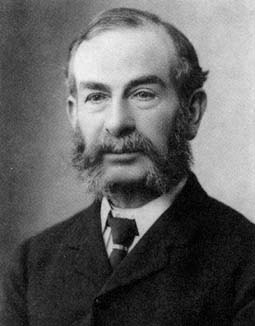
Maxwell's open problem got its answer twice. Edward Routh cracked it algebraically in 1876, and Adolf Hurwitz arrived at an equivalent test independently in 1895. The combined result is the Routh–Hurwitz criterion still taught today. The genius of it: you can certify that every pole sits safely in the left half-plane without ever computing a single pole, just by inspecting the signs in a table built from the polynomial's coefficients.

↘ The math: where the personality comes from

For two complex-conjugate poles written as $s = -\zeta\omega_n \pm j\omega_n\sqrt{1-\zeta^2}$, the transfer function is the canonical second-order form:

$$G(s) = \frac{\omega_n^2}{s^2 + 2\zeta\omega_n s + \omega_n^2}$$

The two pole coordinates map straight onto the two things you feel in the demo. The distance from the imaginary axis is $\zeta\omega_n$, the decay rate, how quickly the response shrinks. The height above the real axis is $\omega_n\sqrt{1-\zeta^2}$, the damped natural frequency, the rate at which the system rings on its way in.

Once the damping ratio reaches $\zeta \geq 1$ the radical $\sqrt{1-\zeta^2}$ goes imaginary, the two poles drop onto the real axis, and the ringing stops entirely. That's the overdamped regime. And the instant any pole crosses into the right half-plane, where the real part $\sigma > 0$, the mode becomes a growing exponential $e^{\sigma t}$ and the response climbs without bound. That is the precise mathematical face of instability.

Everything so far assumes time flows smoothly, but the computer on your robot does not see it that way. It wakes up, samples the sensors, runs the controller, and sleeps, maybe a thousand times a second. That stop-and-go world has its own version of the s-plane, and the stability rule changes shape.

Key takeaways

• Poles (denominator roots) are the system's natural modes; zeros (numerator roots) reshape the response but create no motion of their own.
• A pole's real part sets the decay rate (left is fast, near the axis is sluggish); its imaginary part sets the ringing frequency.
• Stability has one rule: every pole in the left half-plane. One pole in the right half and the whole system diverges.
• Routh and Hurwitz let you check that rule from the coefficients alone, with no pole-solving required.