Bode Plots

Take a transfer function and feed it sine waves of every frequency, from glacially slow to absurdly fast. For each one, the system spits out a sine of the same frequency but a different size and a different timing. Plot the size (gain) and the timing (phase) against frequency, both against a logarithmic frequency axis, and you have a Bode plot, the single most useful picture in classical control.

Drag the s-plane, watch the response

The left panel is the s-plane: drag the pole around and the right panel redraws the gain-and-phase response live. Hover the Bode plot to scrub a single frequency and read off exactly what the system does to it.

Drag the s-plane, watch the Bode plot

reset

show asymptotes off toggle

peak gain —

peak ω (frequency) —

bandwidth (−3 dB) —

poles —

what to try

• Hover the Bode plot: a vertical scrubber annotates $|G(jomega)|$ and $angleG(jomega)$ at that frequency. Find where magnitude is 0 dB.
• Slide a pole leftward (more negative real part). The corner moves to higher $omega$ (frequency). Slower decay = lower bandwidth.
• Drag the conjugate pair toward the imaginary axis. The resonance peak grows. At $zetao0$ (zero damping) it becomes infinite.
• Toggle asymptotes. Each pole contributes one corner and a 90° phase lag; each zero gives a 90° lead. Bode = atoms summed.

Read the two curves like a report card. The gain plot says how loudly the system echoes a given frequency: flat and near 0 dB means "passes through untouched," a downward slope means "this frequency gets squashed." The phase plot says how late the output arrives: every pole eventually drags the phase down by 90 degrees. Where the two curves cross their danger lines tells you how close the closed loop is to ringing itself apart, all without ever solving a differential equation.

The magic is the log axes. On a linear plot, a complicated system is a tangle. On log axes, multiplying transfer functions becomes adding their plots, so a messy product of poles and zeros decomposes into simple straight-line pieces you can sketch and stack by hand. Each real pole is one corner where the gain bends down by 20 dB per decade and the phase leaks away 90 degrees, and each zero is the same move in reverse.

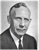
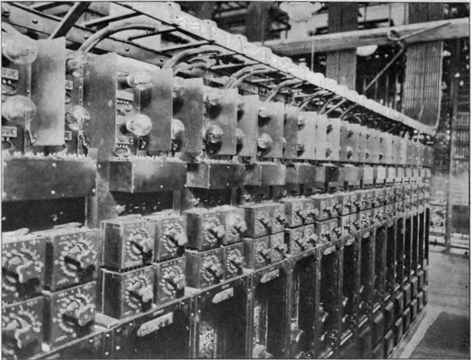
The same math escaped the telephone exchange and went to war. During World War II, Bell Labs engineers, Bode among them, turned this feedback theory loose on fire-control directors, the electromechanical computers that aimed anti-aircraft guns at fast-moving planes. A gun director is a feedback loop too: measure where the target is, predict where it will be, drive the gun there, and try not to overshoot and oscillate. The frequency-domain tools built for keeping phone lines quiet turned out to be exactly the tools for keeping a gun steady, which is one reason the gap between "circuit theory" and "control theory" closed so fast in the 1940s.

↘ The math: substitute s = jω and add up the pieces

Start from the transfer function $G(s)$ and walk straight up the imaginary axis by substituting $s = j\omega$. The complex number $G(j\omega)$ then carries both pieces of the answer at once: its size is the gain, its angle is the phase.

$$|G(j\omega)| = \frac{|N(j\omega)|}{|D(j\omega)|}, \qquad \text{gain (dB)} = 20\log_{10}|G(j\omega)|$$$$\angle G(j\omega) = \arg N(j\omega) - \arg D(j\omega)$$

The reason the log axes are so powerful falls right out of these formulas. Magnitude is a quotient and phase is a difference, so taking the log turns the whole thing into sums: each factor of $G$ adds its own gain curve and its own phase curve independently. A single real pole at $-a$ contributes the factor

$$\frac{1}{1 + j\omega / a}$$

which is flat at low frequency, then breaks downward at the corner $\omega = a$ and rolls off at $-20$ dB/decade while shedding $90$ degrees of phase. A complex pair does the same but twice as steeply, $-40$ dB/decade. Stack the atoms, read the margins, ship the controller.

↘ What the margins are really watching: the −1 point

The two margins are not arbitrary. They both measure distance from one fatal condition. A negative-feedback loop blows up when the signal that comes back around is exactly as big as the signal that went in but flipped in sign, so it reinforces itself instead of correcting. In symbols, with loop gain $\beta A_{OL}$, the danger is

$$\beta A_{OL} = -1,$$

magnitude one and phase $-180$ degrees at the same frequency. This is the Barkhausen criterion, the exact recipe for a circuit that oscillates on its own. The two margins each pin down one half of how far you are from it. Gain margin finds the frequency where the phase has already hit $-180$ degrees and asks how far below unity the gain is there. Phase margin finds the frequency where the gain crosses unity (0 dB) and asks how many degrees of phase you have left before $-180$. If either runs out, you are sitting on the $-1$ point.

How much margin is enough? Stability alone needs the phase margin merely to be positive, but a barely stable loop rings for ages after every nudge. As a rule of thumb, a good step response wants a phase margin of at least $45$ degrees, and engineers often push for $70$ degrees or more when components vary from part to part. There is a catch worth knowing: reading stability straight off the Bode plot only works cleanly for minimum-phase systems, the well-behaved ones with no poles or zeros in the right half-plane. When that fails, you reach for the Nyquist plot instead, which is the next chapter's whole point.

Key takeaways

• A Bode plot is two semi-log graphs (gain and phase versus a logarithmic frequency axis) showing how a system treats slow inputs versus fast ones.
• Log axes turn multiplication into addition, so a complicated response is just simple straight-line pieces added up.
• Gain margin and phase margin, read straight off the plot, tell you how close the loop is to instability: Bode's gift to every controls engineer since the 1940s.