Transfer Functions

The idea is to stop solving the equation and start describing the machine instead. A transfer function $G(s)$ is the system's recipe card: it captures how the plant turns any input into an output, once and for all. Feed it a step, a hammer-blow, a sine wave: the same recipe cooks all three. Below is a textbook second-order plant with two sliders for its character; flip the input picker and watch one recipe produce three completely different dishes.

Same plant, three inputs

Plant G(s) = ω_n² / (s² + 2ζω_ns + ω_n²).

reset

ω_n (natural frequency, how fast) 1.00 ζ (damping, how much it rings) 0.20 ω (input sine frequency, sine only) 1.00

input

step impulse sine

steady-state (step) —

|G(jω)| at picked ω —

∠G(jω) at picked ω —

poles —

what to try

• Step: y settles to 1 (DC gain = 1). The ring around the setpoint is the underdamped response we'll dissect in Lesson 04.
• Impulse: a hammer-blow input. The plant's impulse response is the time-domain twin of its transfer function.
• Sine: now look at the metrics. The steady-state output amplitude matches $|G(jomega)|$ exactly, and the phase lag matches $angleG(jomega)$. This is the bridge to Lesson 05 (Bode).
• With sine mode on, drag the input-ω slider through ω = ω_n. The output amplitude peaks: resonance.

The slider $\omega_n$ sets how fast the plant wants to move; $\zeta$ (zeta) sets how damped it is, how willing it is to ring before settling. Crucially, you never re-derive anything when you change the input. The plant is the plant. That is the whole point: $G(s)$ is a property of the machine, not of what you poke it with.

The magic that makes this possible is the Laplace transform. It takes a differential equation (derivatives, integrals, the works) and turns it into ordinary algebra in a single complex variable $s$. Derivatives become multiplication by $s$; integrals become division by $s$. The fearsome calculus of a robot arm collapses into the kind of polynomial fractions you could push around in high school.

Once you're in that world, the transfer function is just a ratio: $G(s) = Y(s)/U(s)$, output over input, written as a ratio of polynomials in $s$. The bottom polynomial's roots, the poles, tell you everything about stability and ringing. Watch the poles readout in the demo: as you drop $\zeta$, the poles swing toward the imaginary axis and the output rings harder. Push $\zeta$ past 1 and the poles land on the real axis: no ringing, just a lazy crawl to the target.

↘ The variable s is secretly two numbers, and throwing one away gives you the Fourier transform

That single complex variable $s$ is really two real numbers stacked together:

$$s = \sigma + j\omega$$

The $\sigma$ part tracks growth or decay (does the wobble fade or blow up?), and the $\omega$ part tracks oscillation (how fast does it ring?). Most of the time, once you only care about a system that has already settled into a steady hum and you have stopped worrying about the brief turn-on and turn-off transients, you can set $\sigma = 0$. That collapses $s$ down to just $s = j\omega$, a point sliding up and down the imaginary axis.

When you do that, the Laplace transform quietly becomes the Fourier transform: the Fourier transform is just the special case of the Laplace transform with the real part thrown away. That is the exact move the sine probe makes. It is also why frequency response and the Laplace world are not two separate subjects but one subject viewed along a single axis.

Three inputs, one machine

The demo's input picker is the lesson in miniature. Each input probes a different facet of the same $G(s)$:

• Step: switch the input on and leave it. The output settles to the DC gain (here, exactly 1). The wobble on the way up is the underdamped response we dissect in the next lesson.
• Impulse: a single hammer-blow. The output is the plant's impulse response, which is the pure time-domain twin of the transfer function. Hit a bell once and the tone it rings out is its transfer function.
• Sine: drive it with a pure tone and let the transients die. Now the metrics earn their keep: the steady-state output amplitude equals $|G(j\omega)|$ exactly, and the phase lag equals $\angle G(j\omega)$. This is the bridge to frequency response and Bode plots.

Switch to sine mode and drag the input-frequency slider up toward $\omega = \omega_n$. The output amplitude swells dramatically. That's resonance, the same physics that lets an opera singer shatter a glass and that engineers spend careers trying to keep out of bridges and rotor blades.

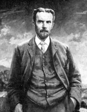
A self-taught telegraph engineer with no university degree, Heaviside treated the derivative operator $d/dt$ as if it were just an algebraic symbol you could multiply, divide, and factor at will. Pure mathematicians were horrified: it had no rigorous justification. Heaviside, busy getting right answers, was unbothered. When pressed on the lack of proof, he reportedly shot back: "Shall I refuse my dinner because I do not fully understand the process of digestion?" The rigor caught up decades later. The engineers had already moved on.

↘ The math: Laplace, the ratio of polynomials, and three special inputs

For a linear time-invariant plant, the output is the convolution of the impulse response with the input. Convolution is brutal in the time domain, but the Laplace transform turns it into plain multiplication:

$$Y(s) = G(s)\,U(s)$$

The transfer function itself is just the output transform over the input transform, written as a ratio of polynomials in the complex variable $s$:

$$G(s) = \frac{Y(s)}{U(s)} = \frac{b_m s^m + \cdots + b_0}{a_n s^n + \cdots + a_0}$$

The second-order plant in the demo is the canonical case, parameterized by natural frequency $\omega_n$ and damping ratio $\zeta$:

$$G(s) = \frac{\omega_n^2}{s^2 + 2\zeta\omega_n s + \omega_n^2}$$

The three inputs are nothing more than three different $U(s)$ multiplied into that same $G(s)$:

$$U_{\text{step}}(s) = \frac{1}{s}, \qquad U_{\text{imp}}(s) = 1, \qquad U_{\text{sine}}(s) = \frac{\omega}{s^2 + \omega^2}$$

Each one picks out a different aspect of $G$. The step's $1/s$ leans on the DC behaviour ($s \to 0$). The impulse's $U(s) = 1$ leaves $G$ bare, so $Y(s) = G(s)$: the impulse response is the transfer function made flesh. And the sine slides $s$ onto the imaginary axis: evaluate $G(j\omega)$ and its magnitude is the gain, its angle is the phase lag. That last move is the entire foundation of frequency-domain control.

↘ Real robots are digital, so they use the z-transform instead

Everything above assumes a smooth continuous-time signal. Real robots do not have one. A microcontroller reads its sensors at a fixed rate, runs a few lines of code, nudges the motors, and waits for the next tick. The signal it sees is a list of samples, $u[0], u[1], u[2], \ldots$, not a curve.

For that world there is a twin of the Laplace transform called the z-transform. It does the same job for sampled signals: it turns a difference equation (this sample plus a bit of the last sample) into algebra in a variable $z$, and you get a discrete transfer function

$$H(z) = \frac{Y(z)}{X(z)}.$$

Here $z$ roughly plays the role of "delay by one sample." The stability test changes shape too. In the $s$-plane safety means staying in the left half. In the $z$-plane it means staying inside the unit circle, $|z| < 1$. Same question (do the poles sit on the safe side of a line?) drawn on a different map. Almost every controller you actually ship runs in this discrete world, because it lives inside a loop on a digital chip.

Key takeaways

• The Laplace transform turns a differential equation into ordinary algebra in a complex variable $s$: derivatives become multiplication by $s$.
• A transfer function $G(s) = Y(s)/U(s)$ is the system's input-output behaviour written as a ratio of polynomials, a property of the machine, not the input.
• The poles (roots of the denominator) decide stability and ringing; left half-plane is safe, right half-plane runs away.
• Step, impulse, and sine are three probes of the same $G(s)$, and the sine probe, $G(j\omega)$, is the doorway to frequency response.