Feedback Control
How a machine argues with reality, and wins, a thousand times a second
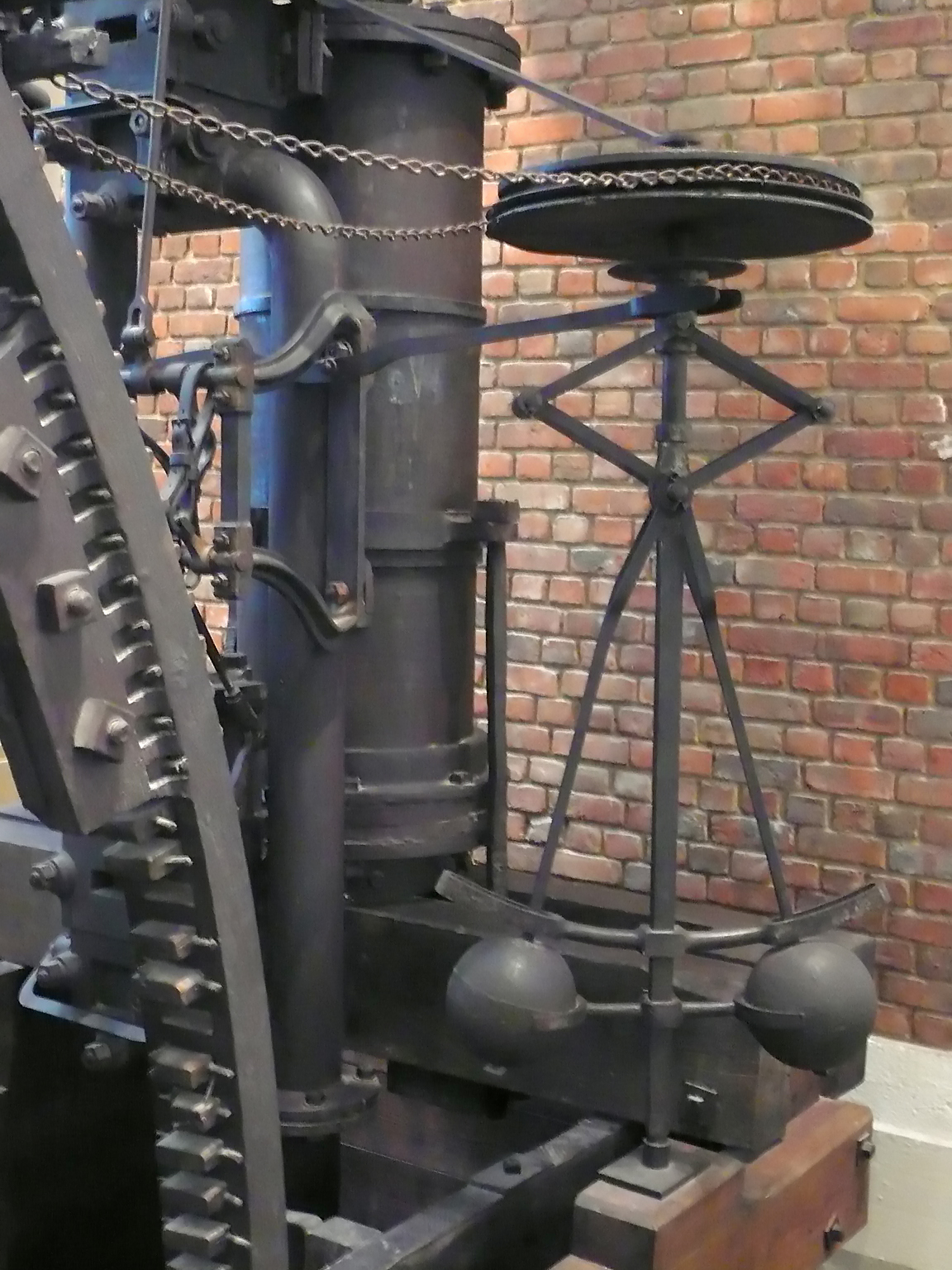
A steam engine has no idea how fast it is going. So in 1788 James Watt bolted on two spinning brass balls that did know, and let them throttle the engine for it.
That gadget is the ancestor of every cruise control, every drone, every thermostat. It is also the simplest idea in all of engineering: measure the mistake, and push back against it.
Send a command and hope: that is open-loop control. Tell the motor “spin at half power” and walk away. It works right up until the floor tilts, the battery sags, or a child sits on the robot. A microwave is open loop: it heats for ninety seconds whether your burrito ends up molten or frozen. Closed-loop control refuses to take the world’s word for it. It measures the actual outcome, compares it to the desired one, and the gap (the error) becomes the next command.
The idea is far older than Watt. People have been measuring mistakes and pushing back against them since antiquity, long before anyone had the math to explain it.
Watch the loop earn its keep
Here are two showers, side by side. The first is open-loop: you set the knob to “what you think 38 °C is” and step in. The second is closed-loop: you feel the water and keep turning. Now slide the real plant gain to simulate calcium creeping into the pipes: the engine has drifted from the model both controllers were tuned for. Watch which one keeps up.
Open-loop vs. closed-loop, when the model is wrong
what to try
- Set Ktrue = 1.0 (the nominal value the controller was tuned for). Both traces hit 1. So far feedback looks redundant.
- Slide Ktrue away from 1.0. The open-loop trace drifts proportionally: its SSE follows the error in K. The closed-loop trace stays glued to 1 (or near it). Robustness.
- Kick the system mid-run. The open-loop controller has no way to notice. The closed-loop one fights back. Without disturbance, you could fake feedback's win with an accurate enough open-loop model. This is the experiment that proves you can't.
- Drop Kp very low (≈ 0.2). The closed-loop response becomes sluggish and underuses its feedback. Crank Kp very high, and it overshoots and oscillates. Two failure modes; the knob you found is the compromise.
The open-loop trace is honest about its weakness. It computes one command from its belief about the plant and commits to it. The moment reality disagrees (K_true slides off 1.0, or a disturbance shoves the output at t = 6 s) it has no way to even notice, let alone respond. The closed-loop trace is forever taking a fresh measurement and leaning back against the error, so it stays glued to the target through gain drift and kicks alike. That stubbornness is called robustness, and it is the entire reason feedback exists.
The single subtraction at the heart of it is the whole game:
where is the reference (where you want to be) and is the measured output (where you actually are). Error drives actuation; actuation changes the output; the new output gets measured; repeat forever. The loop closes.
The bargain: gain for stability
Feedback is not magic; it is a trade. In the demo, drop K_p toward 0.2 and the closed-loop response goes sluggish, barely using the information it works so hard to gather. Crank it sky-high and it overshoots, then overcorrects past the target, then overshoots the other way, louder each time. That runaway is instability, the central hazard of any closed loop. A cruise control gone unstable would surge and brake, surge and brake; a drone’s would wobble itself out of the sky.
The art is to ride the edge: gain high enough to respond crisply, low enough that disturbances decay instead of growing. The knob you settle on is always a compromise between speed, accuracy, and the ever-present risk of the whole thing screaming.
The day feedback got its math
For eighty years feedback was a craft. Watt’s governors worked, but nobody could say why they sometimes hunted and surged instead of settling. The brass balls would catch a rhythm and refuse to let go, the engine speeding and slowing in an oscillation that no amount of tinkering reliably cured.
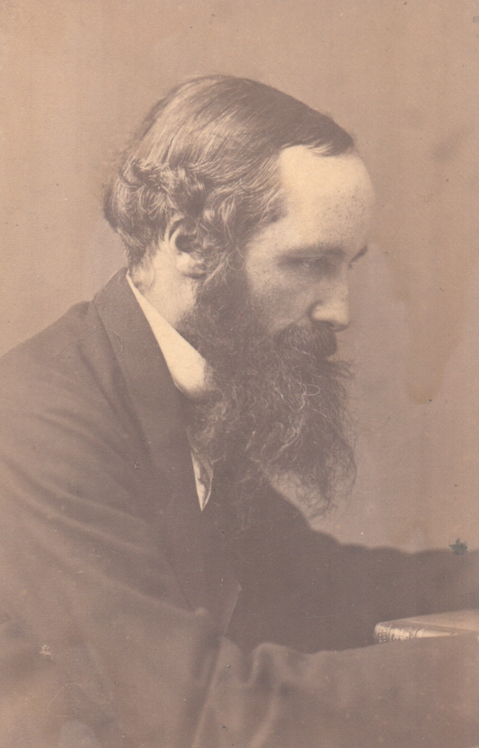
Then in 1868 James Clerk Maxwell (the same Maxwell of the electromagnetic equations) wrote a short paper titled simply On Governors. By treating the governor as a differential equation and asking precisely when its solutions stay bounded, he turned a knack into a science. Stability stopped being luck and became something you could prove on paper before you ever cast a single brass ball.
What Maxwell actually proved, and the friend who finished the job
Maxwell started by sorting the devices into two families. A moderator just drags on the engine like a brake, a centrifugal version of leaning on the pedal. A true governor goes further and adjusts the power going in, so it can hold an exact target speed rather than merely capping it. The clever ones were governors, and the clever ones were the ones that misbehaved.
His insight was that the hunting and surging engineers kept seeing was not bad workmanship. It was baked into the equations. Lags around the loop mean a correction arrives a beat too late, so the governor overshoots, then over-corrects the other way, and the wobble feeds itself. Maxwell wrote down the differential equation for the whole loop and showed that whether the motion settles or grows depends only on the signs of the roots of its characteristic equation. Keep every root’s real part negative and disturbances decay; let one cross into positive territory and the engine oscillates forever. That is the same stability test we still run today, just with poles drawn on a complex plane.
Maxwell worked out the conditions by hand for the low-order cases and admitted the general problem was hard. His old Cambridge classmate Edward Routh picked it up and, in 1874, produced a tidy recipe that checks any order of system without ever solving for the roots. Working separately, Adolf Hurwitz reached the same result, and engineers have called it the Routh-Hurwitz criterion ever since. A craft that began with Ktesibios bailing out a water tank had, in one short generation, become a branch of mathematics.
The math: why a wrong model costs the open loop one-to-one
Both controllers face the same plant, a first-order lag with the real gain and time constant :
The open-loop controller is a single guess: it inverts the gain it believes it has, , and commits.
The closed-loop controller is plain proportional feedback on the live error.
Now follow each to steady state. For the open loop, the output settles at
Any mismatch between the real plant and the model propagates one-to-one into the output. Halve the true gain and you halve the result; the controller never finds out. For the closed loop, the steady-state error works out to
which shrinks toward zero as grows. That is the bargain in symbols: feedback spends loop gain to buy down the error, at the cost of bandwidth and overshoot, the very trade-off the PID controller in the next lesson exists to manage.
Key takeaways
- Open-loop is a wish; closed-loop is a fact. One commits to a guess; the other measures, compares, and corrects, so it survives gain drift and disturbances the open loop can’t even detect.
- The error is the whole engine: it drives actuation, the actuation changes the output, the new output is measured, forever.
- Feedback is a trade: you spend raw gain to buy stability and accuracy, but push too hard and the loop goes unstable.
- Maxwell’s 1868 On Governors turned that trade from craft into provable mathematics.
A machine that runs open-loop is making a wish. A machine that runs closed-loop is having an argument with reality (measure, compare, push back, measure again) and quietly winning it a thousand times a second.
Watt’s brass balls knew it. Maxwell proved it. And every robot you will ever build will live or die by how well it listens to its own mistakes.