Sensing the World
Every robot's reality arrives as a stream of noisy numbers
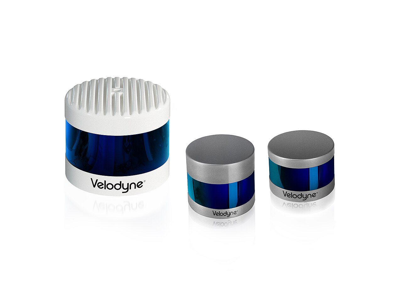
A robot has no eyes, no inner ear, no skin. It has transducers, little devices that turn one kind of energy into a voltage, and that voltage into a number.
Everything the robot will ever believe about the universe arrives through that narrow pipe, and every number in it is slightly wrong.
The job of perception is to take that stream of slightly-wrong numbers and build a usable picture of reality from it. Before we filter, fuse, or map anything, we need a clear-eyed inventory of what kinds of senses a robot can have, and exactly how each one lies.
Here is what that pipe actually looks like, in a real room. A robot slides along the near wall and fires a range beam straight ahead at the far wall, asking “how far?” The dashed beam is the true distance the geometry would give. But the answers that come back (the accent dots) never land exactly on it: each reading is the truth plus a little random error, so they pile up into a cloud of uncertainty sitting right there in space. Turn up the noise σ (the noise level) and the cloud spreads wider; turn up the sample rate and it fills in faster. Watch what happens when the beam swings across the doorway: the true distance jumps long, and so does the reading. The robot only ever sees the dots, never the wall.
The robot slides along the near wall and pings the far wall. The dashed beam is the true distance; each accent dot is one reading, scattered by σ (the noise level). When the beam lines up with the doorway it shoots through and reads long. Bigger σ spreads the cloud; a faster rate fills it in.
The first split: am I sensing me, or the world?
Every sensor falls on one side of a single, load-bearing line.
Proprioceptive sensors measure the robot’s own internal state. A wheel encoder counts how far the axle turned. An inertial measurement unit (IMU) feels its own acceleration and rotation. These sensors need nothing from the outside world (they work in a pitch-black sealed box), and that self-sufficiency is exactly why they are so seductive and so dangerous.
Exteroceptive sensors measure the world beyond the robot’s skin. Lidar, cameras, sonar, a bumper switch: all report something out there. They are the only senses that can tell a robot it has wandered off course, because only they are anchored to something the robot can’t fake.
What a measurement actually says
Sensors also differ in the shape of the fact they hand you. Broadly, there are two flavours.
A range-and-bearing sensor tells you “there is something this far away, in that direction.” A lidar pulse is the purest example: fire a beam, time the echo, multiply by the speed of light, and you have a distance down a known angle. Sonar and radar play the same game with sound and radio. The robot learns geometry (a wall, a cliff, an obstacle) without yet knowing what the thing is.
A landmark sensor instead recognises a specific, identifiable feature: a fiducial tag on a warehouse floor, a labelled corner in a map, a face. Now the robot doesn’t just know something is two metres away; it knows which something. That identity is what lets it pin itself to a map and erase accumulated error in a single observation.
The brutal stopwatch problem hiding inside 'time the echo'
Timing a light pulse sounds simple until you do the arithmetic. Light covers roughly 300,000,000 metres every second. A target sitting 2.5 m away sends its echo back after a round trip of 5 m, which takes about 16.7 nanoseconds:
That is the whole game, and it is unforgiving. If your stopwatch slips by just 10 picoseconds, your distance jumps by 1.5 mm. To put 10 picoseconds in scale: a 3 GHz CPU ticks once every 300 picoseconds, so a single clock tick already smears your reading by 45 mm. Building a sensor that times light to the millimetre means building electronics far faster than the chip running this page.
There are two honest ways to cheat the stopwatch. Direct time-of-flight just races a single sharp pulse and clocks its return, the way a flash lidar lights a whole scene at once. Indirect time-of-flight (the trick inside most depth cameras and the second-generation Kinect) sends out light flickering at a steady rate and measures how far the returning flicker has slipped out of step, then works backward to the delay. Same question, two different ways to read the clock.
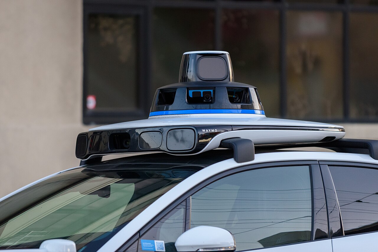
Every sensor lies: pick your poison
Here is the rule that humbles every roboticist: every sensor lies a little, and it lies in three distinct flavours. Confusing them is how robots end up confidently wrong.
- Noise is random jitter. Read the same distance a thousand times and you get a thousand slightly different numbers scattered around the truth. Noise is annoying but honest: it has zero mean, so averaging many readings drives it toward the real value.
- Bias is a constant offset. Your sensor always reads 3 cm too long. Averaging won’t save you; you’ll just converge, beautifully and precisely, on the wrong answer. Bias must be calibrated out, not averaged away.
- Drift is the assassin. It’s a bias that slowly wanders over time, with temperature, with age, with the last bump in the road. A gyroscope reading “zero rotation” while sitting perfectly still will, over minutes, swear the robot is slowly spinning. Integrate that fiction and your sense of “which way is forward” rots without a single alarm going off.
Why drift is so much deadlier than noise
Model a single reading as truth plus three corruptions:
where is a fixed bias, is slowly-varying drift, and is zero-mean noise with variance .
If you average independent readings, the noise term shrinks like the standard error:
So noise is defeatable: collect more samples and it melts away. Bias is constant, so averaging does nothing; it survives untouched and must be measured during calibration.
Drift is worst of all because proprioceptive estimates integrate the signal. A gyro gives angular rate , and heading is its running sum:
A tiny drift in the rate becomes a heading error that grows linearly with time, , and the error in position, which integrates heading again, grows faster still. This is why a great IMU can hold course for a few minutes and then needs an exteroceptive “fix” to survive the hour.
How often must you look? The Nyquist rate
A sensor does not watch the world; it blinks at it, grabbing a reading, then going dark until the next one. Sample too slowly and you do not just lose detail, you can be handed a confident, completely wrong answer.
Picture a wheel spinning fast under a strobe light. Flash it at the right rate and the wheel looks frozen, or even drifts backward. The wheel never changed; your sampling did. The same trap waits for every robot that reads a vibrating, oscillating, or fast-moving signal too rarely.
The rule that saves you is clean and unforgiving. To capture a wave honestly, you must take more than two samples per cycle of the fastest motion in it. Take fewer, and the samples stop pinning the wave down: an impostor wave of lower frequency slips through them just as neatly, and your reconstruction locks onto the impostor. That fake is called an alias, and once it forms, no amount of clever math downstream can tell it from the truth.
Drag A below 2 and watch the signal die:
Drag A. Above 2 samples per cycle the accent reconstruction sits right on top of the true wave. Push A below 2 and the dots no longer pin the wave down: the reconstruction folds to a slower, wrong wave. That is aliasing, and the original signal is gone.
The 2× rule, and the folding that destroys the signal
Write the true signal as a sine at frequency and the sampler as taking samples per second. The Nyquist-Shannon sampling theorem says a signal is perfectly recoverable only if
The threshold is the Nyquist frequency: the highest frequency your sampling rate can honestly represent. Anything above it does not vanish; it folds back below the line. A true frequency sampled at shows up at an apparent frequency
When the nearest multiple is , so and nothing moves. Drop below that and jumps to 1, folding a fast wave down onto a slow one. This is exactly why the demo’s reconstruction collapses to a lazy, wrong wave the moment A crosses 2: every sample still lands perfectly on a slower sine, so a naive reconstruction has no way to know it picked the wrong one.
The practical defence is an anti-aliasing filter: a low-pass filter in front of the sampler that erases everything above the Nyquist frequency before it can fold, so the impostor never gets a chance to form. You throw away the detail you cannot sample honestly, rather than letting it lie to you.
Active vs passive: do you make your own light?
One last axis, and it has real engineering teeth. A passive sensor only receives whatever energy the world happens to send it: a camera waits for ambient photons, a microphone for sound that’s already there. Cheap, silent, low-power, and stealthy. The catch: no light, no data. A passive camera in a dark warehouse is a brick.
An active sensor emits its own energy and measures what bounces back: the lidar’s lasers, sonar’s chirp, a depth camera’s projected dot pattern. It carries its own sun, so it works in total darkness and gives clean range. The price: power draw, cost, and the awkward fact that two active sensors can dazzle each other. A room full of lidars is a room full of robots shouting over one another.
Carrying your own sun has a catch: there is a real sun, and it is much louder than you. A typical depth camera lights the scene with about one watt. Sunlight lands at roughly 1,000 watts per square metre, and even after a narrow optical filter that throws away every colour but the sensor’s own, about 50 watts get through. So on a bright day the sun can outshout the camera’s own signal by something like fifty to one, and the depth image dissolves into glare. This is why a gadget that works flawlessly on your desk can go blind the moment you carry it outdoors.
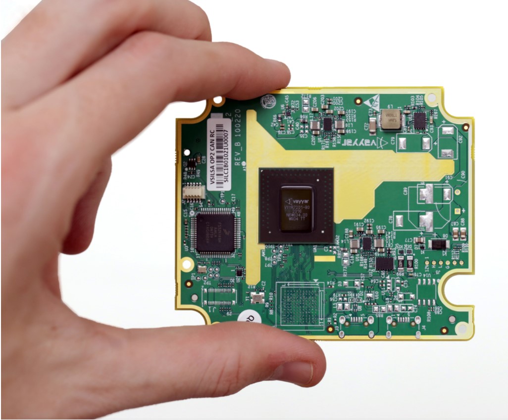
Why a flash lidar barely trips over its neighbours, and how that got a robot onto an asteroid
The “dazzle each other” worry is real for the slow, steady kind of active sensor, but a flash lidar mostly dodges it, and the reason is just arithmetic. A direct flash lidar fires one short pulse, say 10 nanoseconds, and listens for the echo. Light covers 300 metres in a microsecond, so for anything within 100 metres the whole round trip is over in about 660 nanoseconds. The camera only opens its shutter for that brief window, then sits dark until the next pulse. At 30 frames a second the gap between pulses is about 33 milliseconds. So the odds that a second lidar fires exactly while your shutter happens to be open are roughly the open window divided by the gap:
A one-in-fifty-thousand collision is a risk you can live with. That same single-pulse-grabs-the-whole-scene trick is exactly what you want in space, where there is no time to scan dot by dot while you fall toward a rock. A 3D flash lidar of this kind flew on NASA’s OSIRIS-REx mission and helped it reach down and grab a sample from the asteroid Bennu. The same class of sensor has been flight-tested for landing helicopters by themselves. Direct time-of-flight is not just a cheaper depth camera; it is the sense that lets a machine touch a world no one has ever stood on.
Key takeaways
- Proprioceptive vs exteroceptive: sensing your own state (encoders, IMU) versus sensing the world (lidar, cameras). The first never needs the world and never checks against it.
- Range-and-bearing vs landmarks: raw geometry (“something is 2 m away”) versus identity (“that corner is 2 m away”). Identity is what kills drift.
- Noise, bias, drift: random and averagable; constant and calibratable; wandering and lethal. Know which one you’re fighting.
- Active vs passive: make your own energy (works in the dark, costs power, can interfere) or live off the world’s (cheap and quiet, blind without it).
There is no such thing as a robot that perceives the world directly. There is only a machine listening to a chorus of imperfect witnesses (one that drifts, one that’s blind in the dark, one that’s off by a constant inch) and deciding, thousands of times a second, what to believe.
Everything that comes next in this course is the science of believing them well.