01 Foundations & Kinematics · #3 of 46

Robot Kinematics

From joint angles to where the robot actually goes

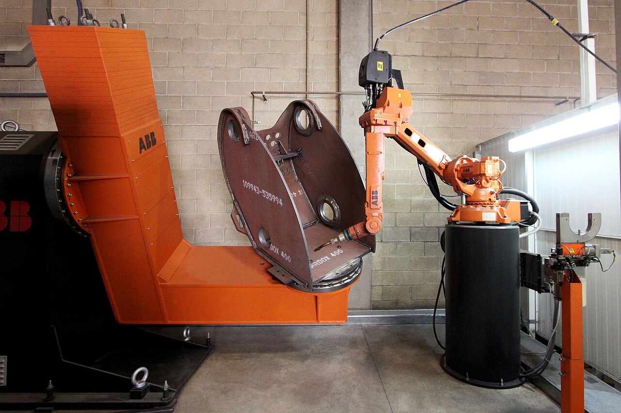
An orange ABB six-axis welding robot bent into a reaching pose. — An ABB six-axis arm: give it the angle of each of its six joints and you know exactly where the torch tip lands. · Ana 2016, CC BY-SA 4.0

Tell this arm the angle of each of its six joints and you can predict exactly where its gripper will be, down to a hair's width. Ask the reverse, "put the gripper there," and the robot has to solve a puzzle that sometimes has eight answers and sometimes has none.

That gap between easy and hard is the whole story of kinematics: the geometry of motion, divorced from the forces that cause it. No mass, no friction, no torque, just shapes and angles and the question if the parts are arranged like this, where does the tip go? Get this right and everything downstream (control, planning, the filters later in this course) has a map to work from.

Forward kinematics: the easy direction

Forward kinematics maps joint angles to the pose of the end-effector: the gripper, the foot, the camera. You feed in the configuration; it hands back a position and orientation. It is easy in the deep sense: there is exactly one answer, and it's a clean chain of multiplications. Set the shoulder, then the elbow, then the wrist; each joint's geometry stacks on the last, and the tip lands wherever the math says. Run it a thousand times a second and you always trust the result.

The Unimate industrial robot arm pouring a cup of coffee in 1967. — Unimate, the first industrial robot, pouring coffee in 1967: installed at GM in 1961, it is the ancestor of every arm whose forward kinematics this lesson describes. · Frank Q. Brown, Los Angeles Times, CC BY 4.0

Try it. This is a three-link planar arm bolted to a base. Drag the three sliders to set each joint angle, $\theta$ (joint angle), and watch the bright end-effector dot land exactly where the chain of links points. Sweep a slider and it leaves a fading trail, the swept tip path; the lightly shaded ring is the reachable workspace, every point the arm can touch. Notice there is only ever one tip for one set of angles: that is forward kinematics, the easy direction. (As a bonus, you can grab the bright tip and drag it directly. The arm now solves the hard direction, inverse kinematics, reaching for your finger.)

end-effector: x 0, y 0

θ₁ 0° θ₂ 0° θ₃ 0°

Drag the joint sliders to sweep, or drag the bright tip to reach a point (inverse kinematics).

Four numbers per joint, since 1955

That "chain of multiplications" needs a rule for how each joint stacks on the last, and for decades there wasn't a standard one. In 1955 two mechanical engineers, Jacques Denavit and Richard Hartenberg, fixed that in a short paper, "A kinematic notation for lower-pair mechanisms based on matrices." Their trick: describe how any one joint connects to the next with just four numbers instead of a full six-number pose. Two of the four say how far and how twisted the link is, the other two say how the joint turns or slides. Pin a little coordinate frame to every joint by their rules and the whole arm becomes a tidy product of matrices. The convention sat mostly unused until Richard Paul showed in 1981 how well it fit computer-controlled robots, and DH parameters have been the default bookkeeping for serial arms ever since.

SCARA: a name that spells out its own geometry

The acronym is the design spec. SCARA stands for Selective Compliance Assembly Robot Arm, and "selective compliance" is the whole trick. The arm is built to be rigid in the vertical direction (so it can press a part down hard and straight) yet a little springy in the horizontal plane (so a peg that lands slightly off-center can still wiggle into its hole). The geometry was worked out in the late 1970s by a team led by Hiroshi Makino at Yamanashi University in Japan, aimed squarely at fast assembly of small electronics. That single goal, snap small parts into place quickly and accurately, fixed every kinematic choice: two parallel revolute joints for quick reach across a flat workspace, plus a vertical slide for the insertion stroke. Design the geometry around the task and the kinematics fall out almost for free.

Inverse kinematics: the hard direction

Now flip the arrow. You know where you want the gripper; you need the joint angles that put it there. This is inverse kinematics, and it is genuinely hard.

The trouble is that the clean one-way street of forward kinematics becomes a tangle going backward. A pose you want might be reachable by many different elbow-up / elbow-down configurations, or by none at all, if it's outside the arm's reach or folded into a place the joints can't twist to. One target, many answers, or zero. The robot has to pick.

Where the magic number eight (and sixteen) comes from

The "up to eight" above is not folklore, it falls out of algebra. Solving inverse kinematics for a serial arm means solving a system of polynomial equations, and a polynomial of degree $n$ has at most $n$ roots. For a fully general arm with six revolute joints, a 6R arm in the jargon, those equations collapse to a single polynomial of degree 16. So a generic 6R arm can present as many as 16 distinct ways to hit one target pose.

Why do real factory arms quote eight, not sixteen? Because most of them aren't built generally. They use an ortho-parallel base and a spherical wrist: the last three joint axes all cross at one point, so the wrist orients without moving the wrist center. That design choice cleaves the 16th-degree problem into something with a clean closed-form answer and at most 8 solutions, which is exactly why engineers picked it. The geometry was chosen to make the inverse problem solvable.

And push the other way: give an arm a seventh joint and you usually get infinitely many solutions for a single pose. The extra freedom is a gift for dodging obstacles, but it means there's no longer a finite list to choose from, so the solver has to optimize rather than enumerate.

The two-link arm: one forward equation, two inverse answers

For a planar arm with link lengths $l_1, l_2$ and joint angles $\theta_1, \theta_2$ , forward kinematics is a direct sum of vectors:

x = l_1\cos\theta_1 + l_2\cos(\theta_1 + \theta_2), \qquad y = l_1\sin\theta_1 + l_2\sin(\theta_1 + \theta_2)

One configuration in, one point out. Inverse kinematics runs it backward. The elbow angle comes from the law of cosines:

\cos\theta_2 = \frac{x^2 + y^2 - l_1^2 - l_2^2}{2\,l_1 l_2}

Notice that $\theta_2$ and $-\theta_2$ give the same cosine. There's your elbow-up and elbow-down pair, two solutions from one target. And if the bracketed value falls outside $[-1, 1]$ , the point is simply out of reach: no solution. That's the whole drama of inverse kinematics in two lines of trigonometry.

Wheels instead of joints

Mobile robots have the same split, but their "joints" are wheels and their "pose" is a spot on the floor. The workhorse model is the differential drive, also called the unicycle: two independently driven wheels on a common axle. Spin them equally and the robot rolls straight; spin them at different rates and it arcs; spin them opposite and it pivots in place.

Differential drive, seen from above, heading right. The right wheel rolls faster than the left, so its arrow v_R is longer. The body velocity v is just their average, and the speed difference bends the path toward the slower left wheel. Extend the common wheel axis and it meets at one pivot: the instantaneous center of rotation (ICR). Spin the wheels at different rates and the robot arcs around it.

This little model matters far beyond cleaning robots. It's the motion model the state estimators later in this course lean on: feed in the two wheel speeds, integrate over a tick of time, and out comes a prediction of the robot's new position and heading. That prediction is the "predict" half of every Kalman filter and particle filter you'll meet, which is why getting the kinematics right is the unglamorous foundation under all the flashy probability.

The unicycle equations the filters integrate

Let the wheels have speeds $v_L$ and $v_R$ , wheel separation $L$ . The robot's forward speed and turn rate are simple averages and differences:

v = \frac{v_R + v_L}{2}, \qquad \omega = \frac{v_R - v_L}{L}

Its pose $(x, y, \theta)$ then evolves by integrating

\dot{x} = v\cos\theta, \qquad \dot{y} = v\sin\theta, \qquad \dot{\theta} = \omega

Two control inputs, $v$ and $\omega$ , yet the state has three numbers. That mismatch is exactly the constraint we name next, and it's why a differential-drive robot can go forward and turn but can never simply slide to its left.

Why you can't slide sideways

Here is the catch hiding in those equations. A differential-drive robot can drive forward and it can rotate, but it cannot move sideways. There is no wheel command for "shift left half a metre." To get there it has to turn, drive, and turn back, exactly the way a car has to parallel-park instead of gliding into the gap.

That property has a name: the robot is nonholonomic. Its instantaneous freedom is smaller than the space it can eventually reach. It can get anywhere on the floor, but not in any direction at any moment: the velocity at each instant is constrained.

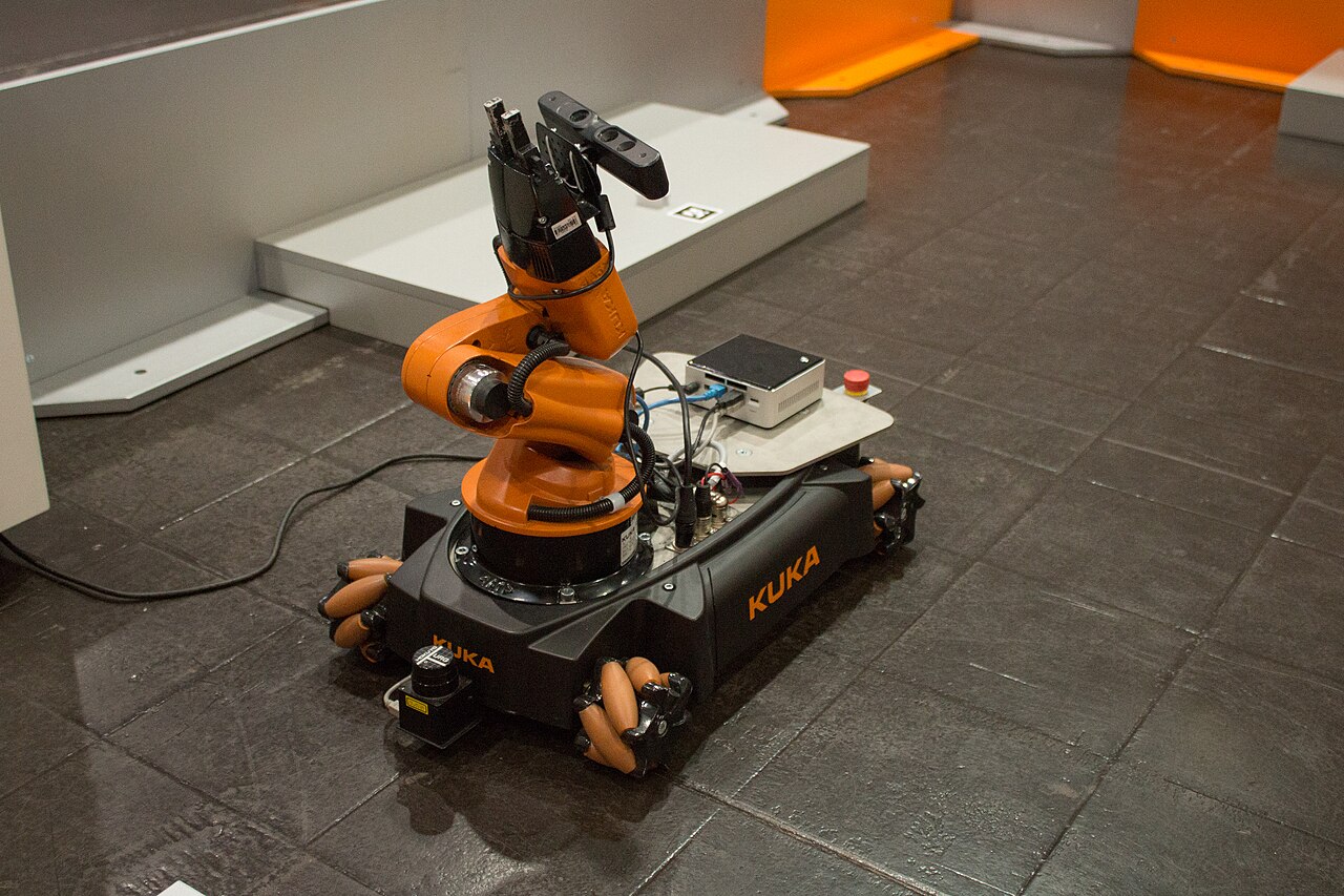
The opposite is holonomic: free to move in any direction at any time, no parallel-parking required. An overhead crane gliding along its rails, or a robot on omnidirectional wheels, can translate straight sideways on command. Holonomic robots are simpler to control and a luxury when you can afford the hardware; most ground robots, like most cars, are stuck being nonholonomic.

A KUKA youBot omnidirectional platform on four mecanum wheels. — A holonomic robot: the KUKA youBot rides on four mecanum wheels whose angled rollers let it slide sideways and spin in place, no parallel-parking needed. · ubahnverleih, CC0

Key takeaways

Forward kinematics maps joint angles to end-effector pose: one answer, easy, a chain of multiplications you can run at full speed.
Inverse kinematics maps a desired pose back to joint angles: hard, with many solutions, or none, plus singularities to dodge.
The differential-drive / unicycle model turns two wheel speeds into motion on the floor; it's the motion model every later filter integrates in its predict step.
A differential-drive robot is nonholonomic: it can't slide sideways, like a car that must parallel-park. Holonomic robots can move any direction at any instant, and pay for it in hardware.

Run forward kinematics yourself

Forward kinematics is just a chain of sines and cosines, and here it is for a two-link arm you can edit. Change the joint angles or the link lengths l1 and l2, run it, and read off where the tip lands.

Forward kinematics of a 2-link arm editable · Python

import math
l1, l2 = 1.0, 0.8
def fk(t1, t2):
  x = l1*math.cos(t1) + l2*math.cos(t1+t2)
  y = l1*math.sin(t1) + l2*math.sin(t1+t2)
  return x, y
for t1, t2 in [(0,0),(math.pi/2,0),(math.pi/4,math.pi/4),(math.pi/2,math.pi/2)]:
  x,y = fk(t1,t2)
  print(f"t1={math.degrees(t1):.0f} t2={math.degrees(t2):.0f} -> ({x:+.2f}, {y:+.2f})")

ready

Kinematics is the quietest subject in robotics and the most load-bearing. Before a robot can decide what to do or wonder where it is, it needs to know what its own body can and cannot do: that the gripper goes there when the joints read this, that the wheels can roll and turn but never slip sideways.

Everything ahead (the planning, the control, the probabilistic guessing-game of state estimation) is built on top of these honest little equations. Master the geometry of motion, and the robot finally has a body it can trust.