06 Path & Motion Planning · #25 of 46

Graph Search & Grid Planning

How a robot finds the shortest way through a world it has never seen

Your GPS, the ghost chasing you through a video-game maze, and a Mars rover all share a secret. Under the hood, they are running the same idea, and one version of it was sketched out, with no paper, in about twenty minutes at a café.

Before a robot can move, it must answer one deceptively simple question: of all the ways from here to there, which one is best? The answer is one of the oldest and most reused ideas in computer science, and it starts by throwing away the real world.

First, turn the world into dots and lines

A robot does not plan over grass, hallways, or Martian regolith. It plans over a graph: a set of nodes (places you can be) joined by edges (moves you can make), each edge carrying a cost (distance, time, energy, risk). Rooms become nodes; doorways become edges. A road map is already a graph; so is a subway diagram.

The floor becomes a graph: places are nodes, moves are weighted edges. "Cross the room" turns into "find the cheapest path from START to GOAL": here, A → C → E → F costs 2 + 6 + 2 = 10.

The most common flavour in robotics is the occupancy grid: chop the floor into squares, mark each as free or blocked, and connect each free cell to its neighbours. That grid is a graph, just a very regular one. Now the messy question "how do I cross the room?" becomes the crisp question "what is the cheapest path through this graph?" And cheapest-path problems, unlike crossing-the-room problems, have algorithms that are provably right.

Dijkstra: flood the room, fairly

The foundational answer is Dijkstra's algorithm. The intuition is almost physical: imagine pouring water at the start node. It spreads outward, always filling the nearest unflooded place next, until it reaches the goal. Because it always expands the cheapest-known node first, the moment water touches the goal, the path it took is guaranteed to be the shortest one. No move can be cheaper than one already considered.

A* · expanded 0 · searching

Click/drag to draw walls. Drag the square (start) or ring (goal) to move them.

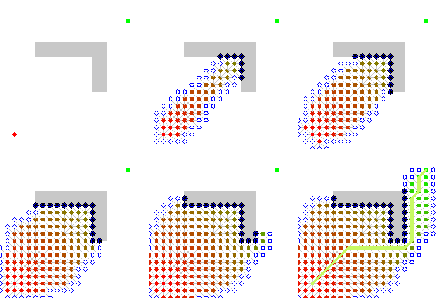
Build a maze and watch it think. Click or drag on the grid to draw and erase walls; drag the start and goal markers anywhere. Toggle between Dijkstra and A* and watch the difference: Dijkstra floods outward in every direction; A* (next section) drives a narrow wedge straight at the goal. Same grid, same answer, wildly different effort.

It is correct and it is complete: if a path exists, Dijkstra finds it, and finds the best one. The flaw is plain in the animation: it spreads in every direction, including straight away from the goal. On a big map that is an enormous amount of wasted searching.

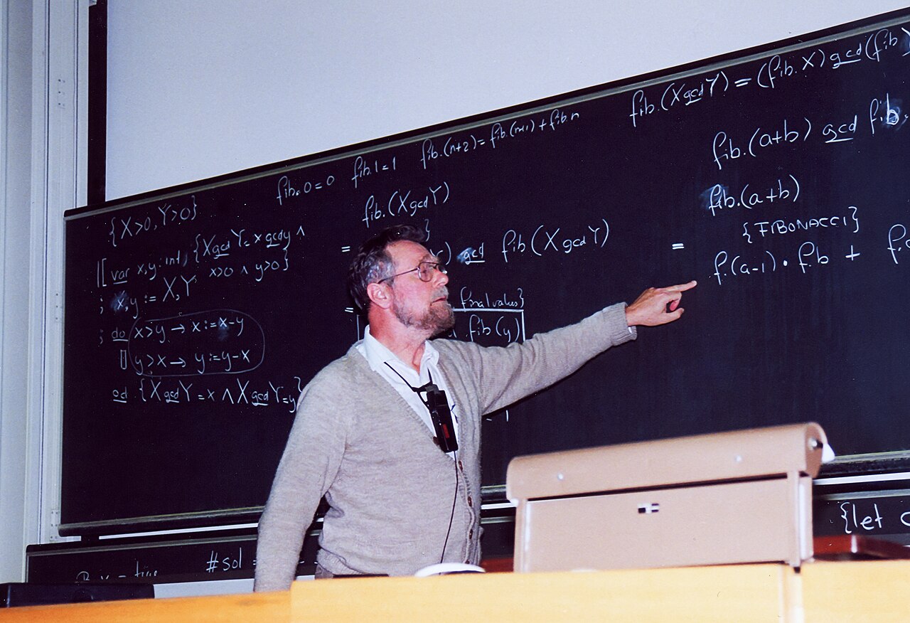
A black-and-white portrait of computer scientist Edsger W. Dijkstra. — Edsger W. Dijkstra · 1930–2002 Designed his shortest-path algorithm in about twenty minutes in 1956, *in his head*, at an Amsterdam café. read more →

He did not invent it for robots, or even really for fun. He had a new computer to show off.

A*: Dijkstra with a hunch

Dijkstra searches blind because it has no sense of direction. A* (pronounced "A-star") fixes exactly that. It keeps Dijkstra's honest accounting of the cost so far (call it $g(n)$ ) and adds a guess of the cost still remaining: a heuristic $h(n)$ . It then always expands the node with the smallest total estimate:

f(n) = g(n) + h(n)

That single added term transforms the search. On a grid, $h(n)$ might be the straight-line distance to the goal: a number you can compute instantly and that ignores all the walls. It pulls the search toward the goal like a compass, so A* explores a slim wedge instead of flooding the whole room. Compare the two animations on this page: same map, same answer, a fraction of the work.

An animated A* search on a grid expanding open and closed nodes outward before tracing the final path to the goal. — Watch A* in motion: open cells (one shade) and closed cells (another) spread from the start, but the heuristic steers them into a narrow wedge until the final shortest path snaps into place at the goal. · Subh83, CC BY 3.0

The famous formula did not arrive in one flash of insight. It was assembled, piece by piece, by three people arguing about how to score a guess.

The fine print: admissible heuristics

Here is the catch that makes A* trustworthy instead of merely fast. The heuristic must be admissible: it must never overestimate the true remaining cost. It is allowed to be optimistic; it is not allowed to be pessimistic.

The reasoning is subtle but worth holding onto. If $h$ never overshoots, then A* can never be tricked into committing to a path before it has ruled out a cheaper one, so with an admissible heuristic, A* is guaranteed to find the shortest path. Straight-line distance is admissible because no route through walls can ever be shorter than flying straight there. Make the heuristic too aggressive (claim the goal is closer than it can possibly be) and A* runs faster but may confidently return a route that is not actually the best. Speed bought with a lie.

The interesting part is that the lie does not have to be reckless. You can tell a measured lie and get a guarantee in return.

Weighted A*: pay a known price for speed, and the memory bill nobody warns you about

The honest trade is called weighted A*. Take an admissible heuristic $h_a$ and inflate it by a factor $\varepsilon > 1$ :

f(n) = g(n) + \varepsilon \, h_a(n).

The search now leans harder toward the goal and expands fewer nodes, so it finishes faster. The catch is bounded, not open-ended: the path it returns is never worse than $\varepsilon$ times the true shortest path. Crank $\varepsilon$ up for speed when "good enough" is fine; drop it back toward 1 for optimal when it is not. That is the principled version of the trade, as opposed to just shrugging and hoping.

There is a second, quieter problem with A*. To guarantee it never misses a better route, A* keeps every node it has generated in memory. On a big map that bill grows fast, and in practice the memory, not the clock, is what kills a naive A* implementation. A whole family of memory-bounded variants exists to fight this, with names like Iterative Deepening A* and SMA* (Simplified Memory-bounded A*), which throw away the least promising nodes when memory runs short and regenerate them later if they turn out to matter.

Why optimism keeps A* optimal, and what 'consistency' buys you

Let $h^*(n)$ be the true cheapest cost from node $n$ to the goal. A heuristic is admissible when

h(n) \le h^*(n) \quad \text{for every node } n.

Suppose A* is about to expand the goal via a suboptimal path of cost $C > C^*$ , where $C^*$ is the optimal cost. Somewhere on the true optimal path sits an unexpanded node $n$ , still waiting in the queue. Because $h$ never overestimates,

f(n) = g(n) + h(n) \le g(n) + h^*(n) = C^*.

So $f(n) \le C^* < C$ , meaning $n$ has a lower estimated total than the bad goal node, and A* would have expanded $n$ first. The contradiction means A* never returns a suboptimal path: it is optimal.

A stronger property, consistency (or monotonicity), demands that for every edge from $n$ to a neighbour $n'$ with cost $c(n, n')$ ,

h(n) \le c(n, n') + h(n').

This is just the triangle inequality applied to estimates. Every consistent heuristic is admissible, and consistency guarantees that once A* expands a node it never needs to revisit it, making the search not only optimal but efficient. Two extremes bracket the design space: set $h(n) = 0$ everywhere and A* collapses back into plain Dijkstra; set $h(n) = h^*(n)$ exactly and A* walks the optimal path without a single wasted expansion.

The two promises every planner makes

When you evaluate any search algorithm, you are really asking two questions:

Completeness: if a path exists, will it definitely be found? Dijkstra and A* both say yes.
Optimality: will the path found be the best one? Dijkstra: always. A*: always, provided the heuristic is admissible.

These are not academic niceties. A delivery robot that is "usually" complete will eventually freeze in a doorway it swears is blocked. An algorithm that is fast but not optimal will quietly burn extra battery on every single trip, forever. The guarantees are the product.

Run the search yourself

Here is Dijkstra's algorithm on the exact graph from the diagram above, and you can edit it. Change a weight in edges and run it again to watch the cheapest route shift. As drawn, it finds A to C to E to F at a cost of 10.

Dijkstra's shortest path editable · Python

import heapq
edges = {'A':[('B',4),('C',2)],'B':[('C',5),('D',3)],'C':[('B',5),('E',6)],
       'D':[('E',1),('F',7)],'E':[('F',2)],'F':[]}
def dijkstra(start, goal):
  dist, prev, pq = {start:0}, {}, [(0,start)]
  while pq:
      d,u = heapq.heappop(pq)
      if u == goal: break
      for v,w in edges.get(u,[]):
          nd = d+w
          if nd < dist.get(v, float('inf')):
              dist[v]=nd; prev[v]=u; heapq.heappush(pq,(nd,v))
  path=[goal]
  while path[-1]!=start: path.append(prev[path[-1]])
  return list(reversed(path)), dist[goal]
path, cost = dijkstra('A','F')
print("cheapest path:", " -> ".join(path))
print("total cost:", cost)

ready

Strip away the lidar, the wheels, the Martian dust, and every path a robot has ever taken comes down to dots, lines, and a willingness to imagine the whole journey before taking the first step.

Dijkstra worked it out in his head in twenty minutes. A* gave that idea a sense of direction and sent it off to guide a clattering robot through a cluttered room. Decades later it is still the quiet voice telling you to turn left in 400 metres: the same beautiful idea, just better at knowing which way to look.