EKF SLAM
How a robot draws the map and finds itself on it at the same time
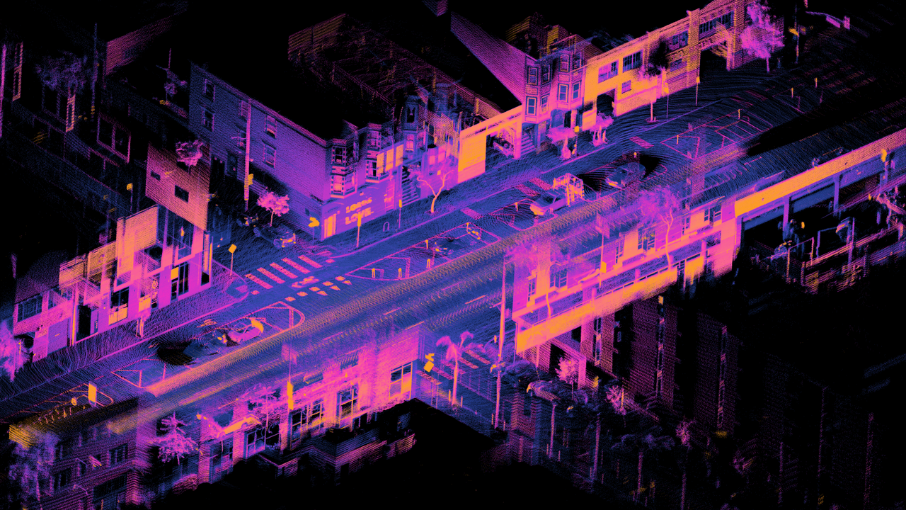
To build a map you need to know where you are. To know where you are you need a map. A robot that has just woken up in an unknown room has neither, and has to bootstrap both at once.
This is the chicken-and-egg problem at the heart of robotics, and for a long time it looked unsolvable. The trick that cracked it is almost embarrassingly simple, and you can watch it happen below.
landmarks 0/0 · loops 0 · robot err 0.00m · map err 0.00m
Yellow = first sighting, green = re-observed. Drive a lap: the estimate (blue trail) drifts from truth, then re-seeing an early landmark snaps the whole map tighter: robot AND landmark ellipses shrink together.
The robot does not know where it is and does not know where the landmarks are. But it knows one precious thing: how far apart it and each landmark are, the instant it looks. Hold onto that: it is the entire secret.
Play with the entanglement
The accent ellipse is the robot’s uncertainty. The blue ellipses are landmark uncertainties. The faint halo is sensor range: anything inside it gets observed this tick.
Try this:
- Drive blind. Move the robot. Watch its uncertainty ellipse swell as odometry drift accumulates, the same drunkard’s walk you met in the last phase.
- First sighting. Spot a brand-new landmark. Its ellipse starts huge, then shrinks within a few looks as the robot triangulates it.
- The magic moment. Drive a loop and return to a landmark you logged way back at the start. The instant you re-recognise it, the entire map snaps tighter at once: robot and every landmark. That is loop closure, and it is the most satisfying half-second in all of SLAM.
- Spot the strings. Watch two nearby landmark ellipses shrink together even when you only looked at one. They are not independent. They never were.
One matrix to bind them
Here is the idea most courses bury under linear algebra. EKF-SLAM does not keep a separate guess for the robot and a separate guess for each landmark. It keeps a single state vector (robot pose stacked on top of every landmark position) and a single covariance matrix that records how every estimate correlates with every other.
That shared matrix is the secret. When you re-observe an old landmark, the correction doesn’t just nudge that one landmark. It flows down the off-diagonal correlations into the robot’s pose, and from there back out into landmarks the robot hasn’t looked at in minutes. The robot and the map are tied together by invisible springs of mathematics. Pull one, and the whole structure heals.
Predict, then correct, now with a map
EKF-SLAM is just the Kalman two-step you already know, run on a state vector that happens to include the world.
Predict. The robot moves. Push the pose through the motion model, and let its uncertainty grow:
where is the Jacobian that linearizes the motion: the “E” in EKF, because the real motion is curved and we pretend, locally, that it is flat.
Update. A landmark comes into view. Compute the Kalman gain, then correct everything by how wrong the prediction was:
Here is the measurement model (the range and bearing the robot expects to see) and is the innovation, the surprise. The genius is that has a row for every state, so a single observation rewrites the robot pose and all the correlated landmarks in one stroke.
The math: why the covariance matrix is the whole map
Stack the robot pose and all landmarks into one state:
The robot pose is ; each is a landmark. The estimate’s uncertainty lives in one big covariance matrix:
The diagonal blocks are how unsure you are about each thing on its own. The off-diagonal blocks (, ) are the springs. They say “if the robot turns out to be a metre east, this landmark must be a metre east too.” Loop closure works because those blocks are non-zero: a measurement of one landmark reaches every estimate it is correlated with.
For a range-and-bearing sensor, the measurement Jacobian (with the offset from robot to landmark and ) is:
Notice it has columns for the robot pose and for the observed landmark. That is the channel through which a single look corrects both ends of the spring at once.
The quadratic cost falls straight out of this picture: a matrix that correlates everything with everything has on the order of entries to maintain. Beautiful, and unscalable.
Where it earns its keep
The hard part in practice is rarely the filter. It is data association: deciding which landmark you’re looking at. Guess wrong, fuse a measurement into the wrong landmark, and the springs yank the whole map into a confident, catastrophic lie. The standard defence is the Mahalanobis distance, which measures “how surprising is this observation, scaled by how uncertain I already am,” and refuses any match beyond a few sigma.
// Mahalanobis distance: accounts for uncertainty
fn mahalanobis_dist(z: Vec2, landmark: Vec2, s: Mat2) -> f32 {
    let innovation = z - landmark;
    (innovation.transpose() * s.inverse() * innovation).sqrt()
}

// Match to nearest landmark within 3-sigma; otherwise it's new
if mahal_dist < 3.0 { /* associate */ } else { /* spawn a landmark */ }
A complete loop subscribes to wheel odometry at high rate for the predict step, to a lidar scan at a lower rate for the update step, extracts landmarks (walls, corners), associates them, and publishes a corrected pose plus a map of landmark positions.
Key takeaways
- SLAM estimates the robot pose and the map simultaneously; neither comes first.
- All of it lives in one covariance matrix; the off-diagonal correlations are the map’s structure.
- Loop closure (re-seeing an old landmark) tightens every estimate at once.
- The elegance costs per update: great for hundreds of landmarks, painful for millions.
A robot waking up in a dark room has no map and no idea where it stands. Within a few seconds it has both, not because it solved the chicken-and-egg problem, but because it refused to choose. It guessed at both, watched how they had to move together, and let one truth pull the other into focus.
Drive a loop, return to where you started, and the whole world clicks into place. That click is the sound of a machine realising it has been somewhere before.