Capstone: Motor Speed Control
Close a PID loop around a real spinning thing and refuse to let the load win
You commanded the drone to hold 6,000 RPM. Then the wind picked up, the blade bit harder air, and the rotor sagged. The drone dipped. Nobody touched the throttle, and yet the speed recovered.
That quiet refusal to lose is the whole point of this chapter. Time to wire it all together around something that actually spins.
A DC motor is the perfect first real target for everything you’ve learned. Feed it voltage and it spins; but its speed is a tug-of-war between that voltage, the friction in its bearings, whatever load you’ve hung off the shaft, and its own back-EMF, the voltage the spinning motor generates against you. Leave it open-loop and the speed drifts the instant any of those change. So we close a PID loop around the first-order motor model from earlier in the chapter and make it hold the line.
Drive the loop yourself
Below is a PI controller wrapped around that motor. The dashed line is the target speed you commanded (6,000 RPM); the solid trace is the actual rotor speed; and at t = 5 s a load torque slams on, like a cordless drill biting into wood. Watch how the speed sags the instant the load hits, then claws its way back to the line.
Hold the RPM under load
what to try
- Set Ki = 0. The motor returns to some speed under load, but not the commanded one. Watch the residual error.
- Bring Ki up. The trace climbs back to the setpoint after each load step. The integrator is doing exactly what its name says: accumulating until the error is gone.
- Ki too high → overshoot during recovery, then oscillation. The PI sweet spot is small-Ki with a Kp that's bigger than the integrator wants it to be.
The story plays out in three acts. The motor spins up and locks onto the target. Then the load hits and the speed plunges, because physics doesn’t care what you commanded. And then, if you’ve tuned it right, the trace climbs stubbornly back to the setpoint, because somewhere inside, an integrator is quietly tallying up every fraction of a second the motor spent too slow and converting that grudge into more voltage.
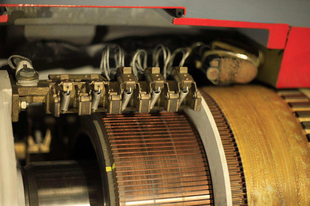
The figure shows a brushed motor, the old workhorse. A ring of copper segments called the commutator spins with the rotor, and two carbon brushes press against it to feed current into the right coil at the right instant. The mechanical switching is the whole trick, but it is also the weak point: the brushes literally rub themselves away. In use the soft carbon wears down to fit the curve of the commutator and keeps wearing, so brushed motors carry a maintenance bill, replace the brushes, clean the commutator, repeat. The brushes in a cheap toy motor are sometimes just a folded strip of springy metal scraping the contacts.
Here’s the key thing to feel in the demo: proportional control alone can hold a speed, but it cannot recover one. Set the integral gain to zero and the motor settles under load, just not at the speed you asked for. It parks at whatever speed makes the proportional push exactly balance the load torque, and that gap never closes. The proportional term only acts on the error that exists right now; a steady offset produces a steady, insufficient push. Only the integrator, accumulating that lingering gap over time, can build enough extra voltage to erase it entirely.
Why this matters everywhere
Speed control is not a toy. The exact loop in the demo (measure speed, compare to target, integrate the error, push harder) runs in places you touch every day:
- Drone rotors, each ESC holding its commanded RPM against gusts and battery sag.
- Hard drives, spinning platters at a rock-steady 5,400 or 7,200 RPM so the read head lands where it expects.
- CNC spindles, holding cutting speed as the tool plunges into metal.
- EV traction motors, delivering smooth torque from a standstill to highway speed.
Different scales, different power, same three-letter loop.
The universal motor: the screaming thing in your corded drill
Plug-in power tools hide a genuinely odd machine called the universal motor, and the name is honest: it runs on either AC or DC. It is a series DC motor, meaning the field winding and the armature carry the same current in series. Here is why that lets it shrug off AC. When the AC mains reverses, the current in the field and the current in the armature both flip at the same instant, and torque is the product of the two. A negative times a negative is still positive, so the shaft keeps pushing the same way no matter which half of the cycle the wall is on.
That one quirk has a wild consequence. An ordinary AC induction motor is chained to the line frequency: its top speed is set by the 50 or 60 hertz coming out of the wall. A universal motor is not, so it can spin far faster than that synchronous limit. High speed means a lot of power from very little metal, which is exactly why a drill, a router, a circular saw, and a vacuum cleaner all use one. They are loud and they wear their brushes, but they are light and they are cheap. The downside is the series wiring: a series motor must never run with no load. Unloaded, the current drops, the back-EMF goes weak, and the motor speeds up trying to balance the supply voltage, faster and faster, until it can tear itself apart. Bench grinders and drills lean on the friction of the work to keep that in check. Commercial universal motors are usually small, under about a kilowatt, but engineers once built huge ones to pull electric locomotives, fed by special low-frequency power lines to keep the commutator from arcing under the load.
Three ways to wire a DC motor, and the second speed knob nobody mentions
A wound DC motor has two sets of windings, the field on the stationary part and the armature on the spinning part, and how you connect them sets the motor’s whole character. There are three classic choices. Wire the field and armature in series and you get the muscle motor above: huge starting torque, speed that sags hard with load. Wire them in parallel, the shunt connection, and the field sees the full supply no matter what the armature is doing, so the speed barely budges as the load changes. That steady speed is why shunt motors ran machine tools and winding machines for a century. Splice the two together and you get a compound motor, which borrows the strong start of a series winding and the steady speed of a shunt one.
Here is the part most people miss. Armature voltage is not the only speed knob. Speed is set by the ratio of voltage to field strength, so you can also speed a motor up by weakening the field, dialing down the current in the field winding. It feels backwards, fewer amps in the magnet making the thing spin faster, but it falls right out of the back-EMF balance: a weaker field needs more RPM to generate the same opposing voltage. Big industrial drives, like the separately excited motors that once ran mine hoists on thyristor controllers, used voltage control down low and field weakening up high to cover a huge speed range. Those have mostly been swapped for AC motors on variable-frequency drives now, but the trick lives on in how EV traction motors stretch a single gear ratio across the whole speed band.
The tuning dance, one last time
The demo lets you feel the PI trade-off directly:
- Ki = 0: pure proportional. The motor recovers to a speed after the load, but a stubborn residual error remains. Read it off the “SSE after load” metric.
- Bring Ki up: the trace climbs all the way back to the setpoint after each load step. Watch “recovery time” shrink.
- Ki too high: recovery overshoots, then the speed rings and oscillates. The sweet spot is a modest integral gain with a proportional gain bigger than the integrator alone would want.
The math: a first-order motor plant and the PI law
A DC motor’s speed obeys a clean first-order torque balance. The driving torque from the input fights viscous friction and any external load torque , all divided by the rotor inertia :
With no load and constant input this settles to a steady speed, and the input-to-speed relationship is the canonical first-order lag, with gain and time constant :
We close the loop on the error (commanded speed minus actual) with a PI controller, proportional plus integral. The derivative term is dropped because speed measurements are noisy and a load step needs erasing, not anticipating:
Now the punchline. A constant load torque is a step disturbance. Plug it into the closed loop and ask for the steady-state error using the final-value theorem. With the error settles to a nonzero value proportional to the load, the residual you saw in the demo. With any , that integrator contributes a pole at the origin (an in the denominator of the open loop), which forces the steady-state error from a step disturbance to exactly zero. That is the entire mathematical reason the integrator recovers the speed and the proportional term cannot. The demo integrates the plant and controller together by forward-Euler at , with the load torque switching on at .
Key takeaways
- A DC motor’s speed is a fight between voltage, friction, load and back-EMF. Closing a PID loop around the first-order motor model holds it steady through all of them.
- Proportional can hold a speed but leaves a residual offset under load; integral is what recovers the commanded speed after a disturbance, by driving steady-state error to zero.
- Watch for integral windup when the actuator saturates: the integrator’s long memory becomes a liability.
- This same speed loop runs drone rotors, hard drives, CNC spindles, and EV traction motors.
A motor, a load that fights it, and three numbers that refuse to lose. That’s the capstone.
Everything in this chapter pointed here: the error, the three terms, the trade-off between speed and stability. Now you’ve closed the loop around something that spins, shoved a disturbance at it, and watched the integrator quietly win the argument. The next time a drone holds altitude in a gust or a spindle holds its speed through a cut, you’ll know exactly which term is doing the stubborn work.